Fitting and Interpreting CART Regression Trees

hacking skills

Author

zenggyu

Published

2018-04-27

Abstract

Shows how to fit and interpret a CART regression tree model.

Introduction

In a previous post, I introduced the theoretical foundation behind regression trees based on the CART algorithm. In this post, I will put the theory into practice by fitting and interpreting some regression trees in R.

About the data set

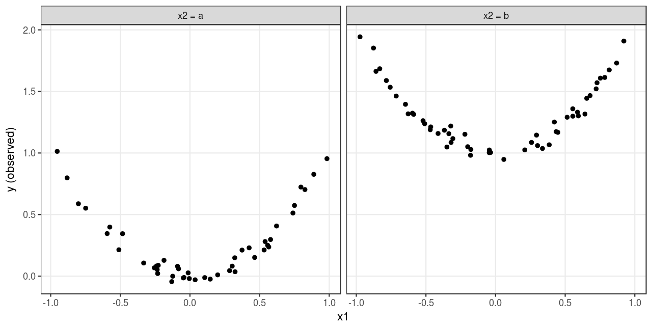
Consider a regression problem. Suppose the outcome \(y\) is a quadratic function of a continuous feature \(x_1 \in [-1, 1]\), a discrete feature \(x_2 \subseteq \{a, b\}\) and an irreducible error \(\epsilon \sim N(0, 0.05^2)\), which takes the following form:

\[ \begin{equation} y = \begin{cases} x_1^2 + 0 + \epsilon, \quad x_2 = a \\ x_1^2 + 1 + \epsilon, \quad x_2 = b \\ \end{cases} \quad (1) \end{equation} \]

A data set (with 100 observations) that reflects the above definition can be simulated using the following code:

library(tidyverse)
library(caret)
library(rattle)
set.seed(1) # For reproducible results.
size <- 100
dat <- tibble(
  x1 = runif(size, min = -1, max = 1),
  x2 = factor(sample(c("a", "b"), size, replace = T), levels = c("a", "b")),
  e = rnorm(size, sd = 0.05),
  y  = x1 ^ 2 + if_else(x2 == "b", 1, 0) + e
)

A visualization of the simulated data set is given in Figure 1:

Fitting regression trees on the data

Using the simulated data as a training set, a CART regression tree can be trained using the caret::train() function with method = "rpart". Behind the scenes, the caret::train() function calls the rpart::rpart() function to perform the learning process. In this example, cost complexity pruning (with hyperparameter cp = c(0, 0.001, 0.01)) is performed using leave-one-out cross validation.

There are some other parameters worth mentioning. The dots parameter (i.e., ...) of the caret::train() function can capture additional arguments, which are then passed to the workhorse function to control its behavior. In this example, the control parameter is, as the name indicates, control. This parameter should be set using the rpart::rpart.control() function, and the following settings may be of particular interest since they determine when to stop splitting.

minsplit: the minimum number of observations that must exist in a node in order for a split to be attempted;
minbucket: the minimum number of observations in any terminal node;
maxdepth: the maximum depth of any node of the final tree, with the root node counted as depth 0.

In this example, the trees are trained with minsplit = 20, minbucket = 7 and maxdepth = 30, which are the defaults.

model <- train(y ~ x1 + x2, method = "rpart", data = dat,
               trControl = trainControl(method = "LOOCV"),
               tuneGrid = data.frame(cp = c(0, 0.001, 0.01)),
               control = rpart::rpart.control(minsplit = 20,
                                              minbucket = 7,
                                              maxdepth = 30))

Interpreting the results

Text output

Here’s the result of the cross-validation process:

model

#> CART 
#> 
#> 100 samples
#>   2 predictors
#> 
#> No pre-processing
#> Resampling: Leave-One-Out Cross-Validation 
#> Summary of sample sizes: 99, 99, 99, 99, 99, 99, ... 
#> Resampling results across tuning parameters:
#> 
#>   cp     RMSE       Rsquared   MAE       
#>   0.000  0.1395381  0.9441324  0.09897355
#>   0.001  0.1401764  0.9434928  0.10082041
#>   0.010  0.1555449  0.9303871  0.12178135
#> 
#> RMSE was used to select the optimal model using the smallest value.
#> The final value used for the model was cp = 0.

As is indicated by the root mean squared error (RMSE), the pruned trees (with cp = 0.001 or cp = 0.01) actually yields worse predictions than the unpruned tree (with cp = 0)¹. Therefore, the final model is the unpruned tree:

¹ This is because the variation attributed to random noise is relatively small, compared with the variation attributed to the underlying pattern.

model$finalModel

#> n= 100 
#> 
#> node), split, n, deviance, yval
#>       * denotes terminal node
#> 
#>  1) root 100 34.688070000 0.82292600  
#>    2) x2b< 0.5 46  3.697102000 0.25443380  
#>      4) x1< 0.6002265 39  2.048577000 0.17957170  
#>        8) x1>=-0.4082083 31  0.305459500 0.08868443  
#>         16) x1< 0.3490279 23  0.063726560 0.03816711  
#>           32) x1>=-0.1585103 16  0.040280410 0.02069034 *
#>           33) x1< -0.1585103 7  0.007388877 0.07811400 *
#>         17) x1>=0.3490279 8  0.014285940 0.23392170 *
#>        9) x1< -0.4082083 8  0.494750500 0.53175980 *
#>      5) x1>=0.6002265 7  0.212215300 0.67152240 *
#>    3) x2b>=0.5 54  3.460525000 1.30719700  
#>      6) x1>=-0.6801389 47  2.193850000 1.25235400  
#>       12) x1< 0.6483196 38  0.562510900 1.16641300  
#>         24) x1< 0.4038528 29  0.383423800 1.13220600  
#>           48) x1>=-0.3583761 19  0.083832340 1.06522800 *
#>           49) x1< -0.3583761 10  0.052415770 1.25946200 *
#>         25) x1>=0.4038528 9  0.035809750 1.27663700 *
#>       13) x1>=0.6483196 9  0.165642400 1.61521800 *
#>      7) x1< -0.6801389 7  0.176157400 1.67542700 *

Tree plot

The final model can be visualized using the fancyRpartPlot() function²:

² The fancyRpartPlot() function comes from the rattle package. On a Debian-based platform (including Ubuntu), it has a system dependency, i.e., the libgtk2.0-dev package, which can be installed using the apt command in a bash session.

fancyRpartPlot <- function (model, main = "", sub, caption, palettes, type = 2,
    ...)
{
    if (missing(sub) & missing(caption)) {
        sub <- paste("Rattle", format(Sys.time(), "%Y-%b-%d %H:%M:%S"),
            Sys.info()["user"])
    }
    else {
        if (missing(sub))
            sub <- caption
    }
    num.classes <- length(attr(model, "ylevels"))
    default.palettes <- c("Greens", "Blues", "Oranges", "Purples",
        "Reds", "Greys")
    if (missing(palettes))
        palettes <- default.palettes
    missed <- setdiff(1:6, seq(length(palettes)))
    palettes <- c(palettes, default.palettes[missed])
    numpals <- 6
    palsize <- 5
    pals <- c(RColorBrewer::brewer.pal(9, palettes[1])[1:5],
        RColorBrewer::brewer.pal(9, palettes[2])[1:5], RColorBrewer::brewer.pal(9,
            palettes[3])[1:5], RColorBrewer::brewer.pal(9, palettes[4])[1:5],
        RColorBrewer::brewer.pal(9, palettes[5])[1:5], RColorBrewer::brewer.pal(9,
            palettes[6])[1:5])
    if (model$method == "class") {
        yval2per <- -(1:num.classes) - 1
        per <- apply(model$frame$yval2[, yval2per], 1, function(x) x[1 +
            x[1]])
    }
    else {
        per <- model$frame$yval/max(model$frame$yval)
    }
    per <- as.numeric(per)
    if (model$method == "class")
        col.index <- ((palsize * (model$frame$yval - 1) + trunc(pmin(1 +
            (per * palsize), palsize)))%%(numpals * palsize))
    else col.index <- round(per * (palsize - 1)) + 1
    col.index <- abs(col.index)
    if (model$method == "class")
        extra <- 104
    else extra <- 101
    rpart.plot::prp(model, type = type, extra = extra, box.col = pals[col.index],
        nn = TRUE, varlen = 0, faclen = 0, shadow.col = 0,
        fallen.leaves = TRUE, branch.lty = 3, ...)
    title(main = main, sub = sub)
}

fancyRpartPlot(model$finalModel, sub = NULL)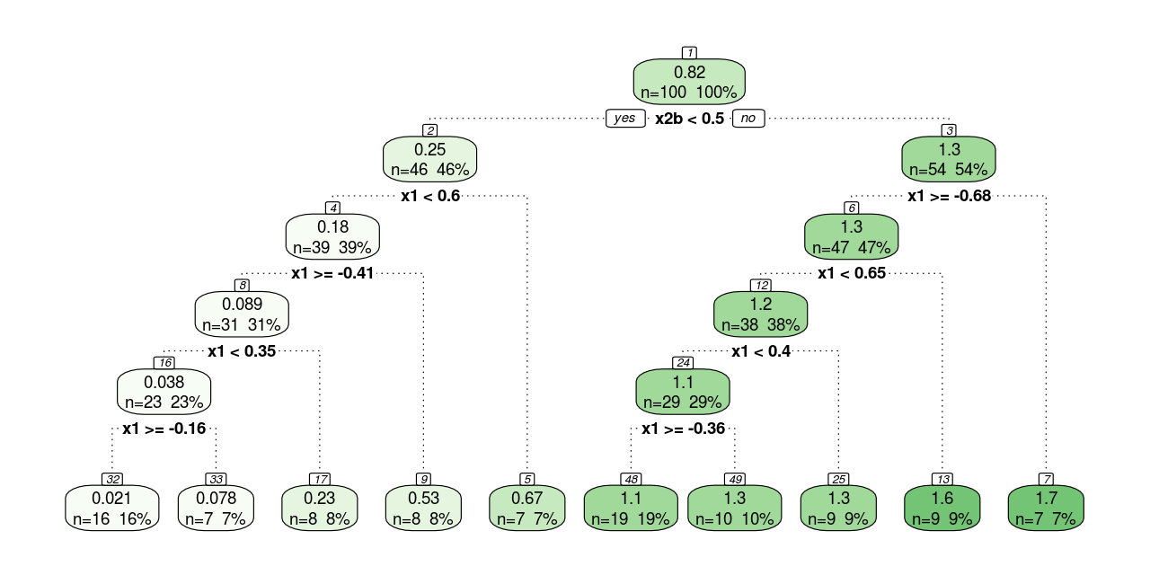

The unpruned tree is plotted in Figure 2 . Every round square box represents a node, and the number at the top of it denotes the ID of the node. The number on the first line of the box is the mean of the outcome of all the observations in that node (if it is a leaf node, the mean is used for prediction); and the higher the mean, the greener the box. The text on the second line shows the sample size in that node. The splitting process begins with a root node at the top and ends with leaf nodes at the bottom. Each parent node is split into two child nodes, and the association is denoted by dotted lines. A condition for each split is presented under parent nodes. Observations that meet the condition (i.e., when the condition yields an answer of “yes”) go to the child node on the left, otherwise go to the child node on the right. Finally, 10 leaf nodes are included in the tree (note how the result complies with the control parameters minsplit = 20, minbucket = 7 and maxdepth = 30).

The splitting conditions for the continuous feature (i.e., x1) are straightforward. However, those for the discrete feature (i.e., x2) need some additional explanation. Before the learning process, the CART algorithm would decompose discrete features into binary dummy variables. By assuming a reference level, a discrete feature with \(n\) possible values can be decomposed into \(n - 1\) binary dummy variables. In this example, \(x_2 = a\) is taken as the reference level, and x2 is decomposed into one dummy variable x2b, which equals 1 if x2 = "b", and 0 otherwise³.

³ Therefore, formula (1) can be rewritten as \(y = x_1^2 + x_{2b} + \epsilon\), which is more convenient for computation.

Predictions

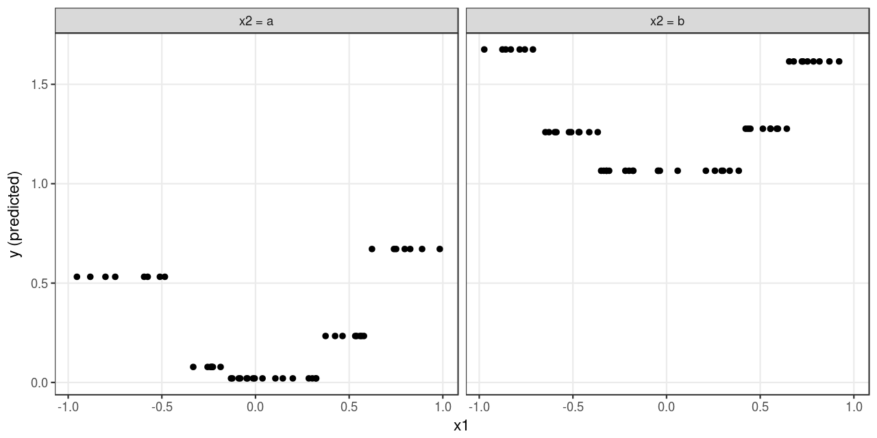
The predicted outcomes are plotted in Figure 3 . The tree model yields an identical prediction for all observations that fall in the same leaf node, which approximates the underlying pattern (see Figure 1 ) loosely. It would require a larger sample size to get a more precise approximation⁴.

⁴ A parametric model (e.g., linear regression with quadratic terms) would approximate the underlying pattern well even with a relatively small sample size.

Variable importance

By keeping track of the overall reduction in the optimization criteria (i.e., sum of squared error, SSE) for each feature, an aggregate measure can be computed to indicate the importance of each feature in the model. This measure is called variable importance, and it is stored in the finalModel object.

model$finalModel$variable.importance

#>       x2b        x1 
#> 27.530443  8.867288

The measure shows that x2b and x1 respectively contribute to the overall reduction of SSE by 27.53 and 8.87. Therefore, x2b plays a more important role than x1 in explaining the variance in the data. Generally speaking, features that appear higher in the tree (i.e., earlier splits) or those that appear multiple times in the tree will be more important than features that occur lower in the tree or not at all.

Here I try to calculate the importance measure for x2b manually, just to make sure I understand the concept correctly. As is shown in Figure 2 , there’s only one split using x2b, which is the first split in the tree. Before the split, the SSE is:

sum((dat$y - 0.82) ^ 2)

#> 34.68893

After the split, the SSE becomes:

sum((dat[dat$x2 == "a",]$y - 0.25) ^ 2) + sum((dat[dat$x2 == "b",]$y - 1.3) ^ 2)

#> 7.161328

Therefore, the overall reduction in SSE attributed to x2b is \(34.68893 - 7.161328 = 27.5276 \approx 27.530443\).

More on the pruning process

The full tree shown in Figure 2 is obtained with cp = 0 and therefore no nodes are collapsed due to cost-complexity pruning. But as the hyperparameter cp increases, more nodes get collapsed, and the resulting tree becomes smaller. The process begins with parent nodes of leaf nodes and ends with the root node. For example, when cp = 0.001, node 16 collapses and becomes a leaf node. When cp = 0.01, node 8, which is the parent node of node 16, collapses and becomes a leaf node; besides, node 12 also collapses and becomes a leaf node.