How to Simulate Data Based on The Assumptions of Logistic Regression

Abstract

Shows how to make simulated data for logistic regression.

Introduction

The main purpose of this post was to show how to simulate data under the assumptions of logistic models. The technique introduced should also be useful for generating simulated data to study other machine learning algorithms.

But before the simulation, I will first introduce some key concepts of logistic regression.

About the logistic function

The logistic regression uses the logistic function to denote the probability of the occurrence of an outcome \(Y = 1\), given an input \(X\):

\[ \begin{align} p(X) &= \frac{e^{X}}{e^{X} + 1} \\ &= \frac{1}{1 + e^{-X}} \end{align} \quad (1) \]

It is apparent that the probability has a positive association with \(X\), and \(p = 1\) when \(X\) approaches \(+\infty\), \(p = 0\) when \(X\) approaches \(-\infty\). It is also worth noting that when \(X > 0\), \(p > 0.5\) and the occurrence of the event is therefore predicted.

The input \(X\) can include one or more predictors, and the combination of the predictors can be linear or non-linear. For instance, if \(X\) is a linear function of one predictors \(x_1\), then \(X\) can be represented as \(\beta_1 x_1\). Typically, \(X\) also includes an intercept term \(\beta_0\), so that \(X = \beta_0 + \beta_1 x_1\). Then the logistic function for this instance becomes:

\[ p(X) = \frac{1}{1 + e^{-(\beta_0 + \beta_1 x_1)}} \quad (2) \]

Abouth the logit function

The logistic function provides a good representation of the relationship between the probability of an outcome and its predictors, but it does not provide a straightforward interpretation of the coefficients (\(\beta_0, \beta_1, etc\)). An alternative representation of the relationship which makes the interpretation a lot easier is the logit function.

The logit¹ (log odds) function (denoted by \(g\) below) is the inverse of the logistic function, which takes the following form:

¹ The term “logit” is an abbreviation for “logistic unit”

\[ \begin{align} g(p(X)) &= ln(\frac{p(X)}{1 - p(X)}) \\ &= X \\ \end{align} \quad (3) \]

Note that \(\frac{p(X)}{1 - p(X)}\) is the odds of the occurrence of the outcome. By exponentiating the terms, we get:

\[ \begin{align} \frac{p(X)}{1 - p(X)} &= e^X \\ \end{align} \quad (4) \]

The above formula provides a straightforward interpretation for the coefficients in \(X\). For example, still asumming \(X = \beta_0 + \beta_1 x_1\), then every 1-unit increase in \(x_1\) will result in the multiplication of the odds by \(e^{\beta_1}\). \(e^{\beta_1}\) can also be seen as the ratio of the odds between two groups of observations where there’s only 1-unit difference in \(x_1\). In this case, \(e^{\beta_1}\) is said to be the odds ratio, which approximates the risk ratio² when \(p(X)\) is small.

² Risk ratio, abbreviated as RR, is the ratio of the probability of an event occurring in a group of observations to the probability of the event occurring in another group of observations.

About maximum likelihood estimation

Logistic regression uses maximum likelihood estimation to estimate the coefficients in \(X\). See the wiki page for more details.

An experiment to simulate data for logistic regression

In this example, I simulate a data set with known distribution and fit a logistic regression model to see how close the result is to the truth.

Consider the probability of an event given input \(X\), as indicated by formula (1). Suppose \(X = -2 + 3x_1^2 + x_2 + \epsilon\), where \(x_1 \in [-1, 1]\) is continuous, \(x_2 \in \{0, 1\}\) is binary (categorical) and \(\epsilon \sim N(0, 0.1^2)\) is random noise. Then formula (1) becomes:

\[ p(X) = \frac{1}{1 + e^{-(-2 + 3x_1^2 + x_2 + \epsilon)}} \quad (4) \]

A data set that reflects the above definition can be simulated with the following code:

library(tidyverse)
set.seed(1)
sample_size <- 300
dat <- tibble(
  x1 = runif(sample_size, min = -1, max = 1),
  x2 = rbinom(sample_size, 1, 0.5),
  e = rnorm(sample_size, sd = 0.1),
  p = 1 / (1 + exp(-(-2 + 3 * x1^2 + x2 + e))),
  log_odds = log(p / (1 - p)),
  y = rbinom(sample_size, 1, p)
)

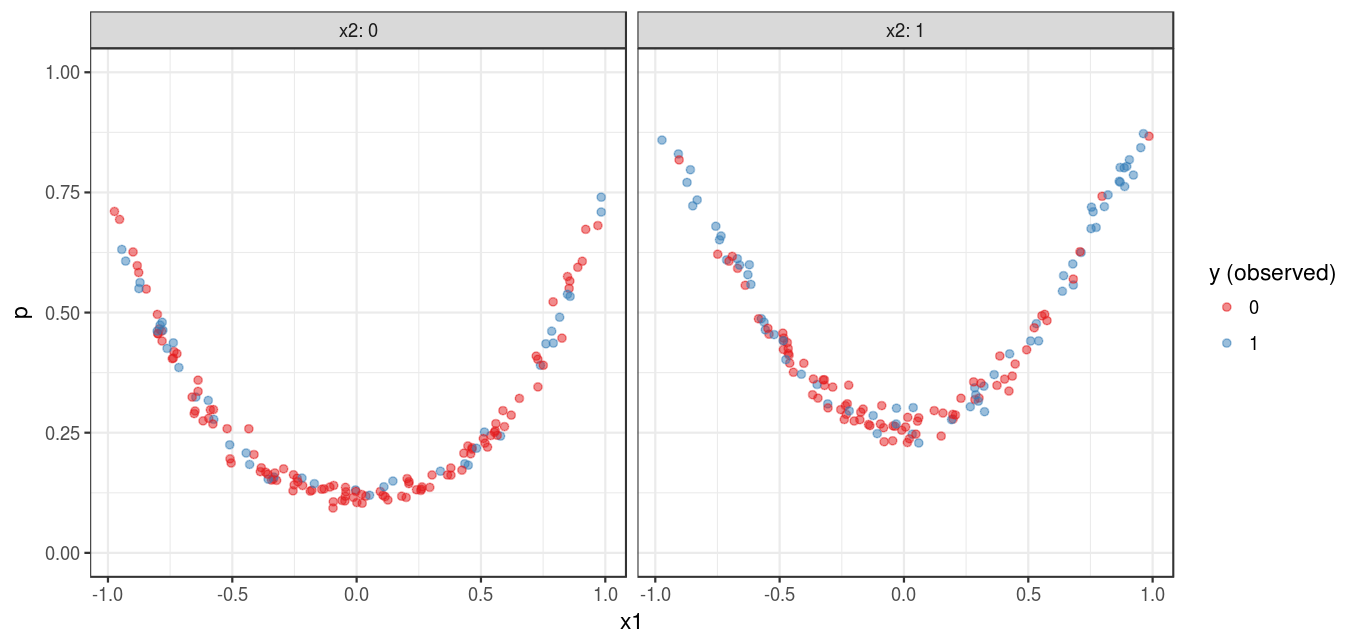
Figure 1 shows the simulated data set with the probability of the event in the y-axis.

Figure 1: Simulated data

Now, let’s fit a logistic model on the data using the glm() function. Note how a quadratic term of x1 is represented in the formula to reflect the underlying definition.

fit <- glm(y ~ I(x1^2) + x2, data = dat, family = binomial)

fit

#> 
#> Call:  glm(formula = y ~ I(x1^2) + x2, family = binomial, data = dat)
#> 
#> Coefficients:
#> (Intercept)      I(x1^2)           x2  
#>      -2.070        2.747        1.088  
#> 
#> Degrees of Freedom: 299 Total (i.e. Null);  297 Residual
#> Null Deviance:       388.5 
#> Residual Deviance: 342.2     AIC: 348.2

The result shows that \(X = -2.070 + 2.747x_1^2 + 1.088x_2^2\), which is fairly close to the truth (i.e., \(X = -2 + 3x_1^2 + x_2\)).

The predict() function can be used to get the predicted probability, which can then be used to get the prediction.

dat <- dat %>%
  mutate(p_predicted = predict(fit, type = "response"),
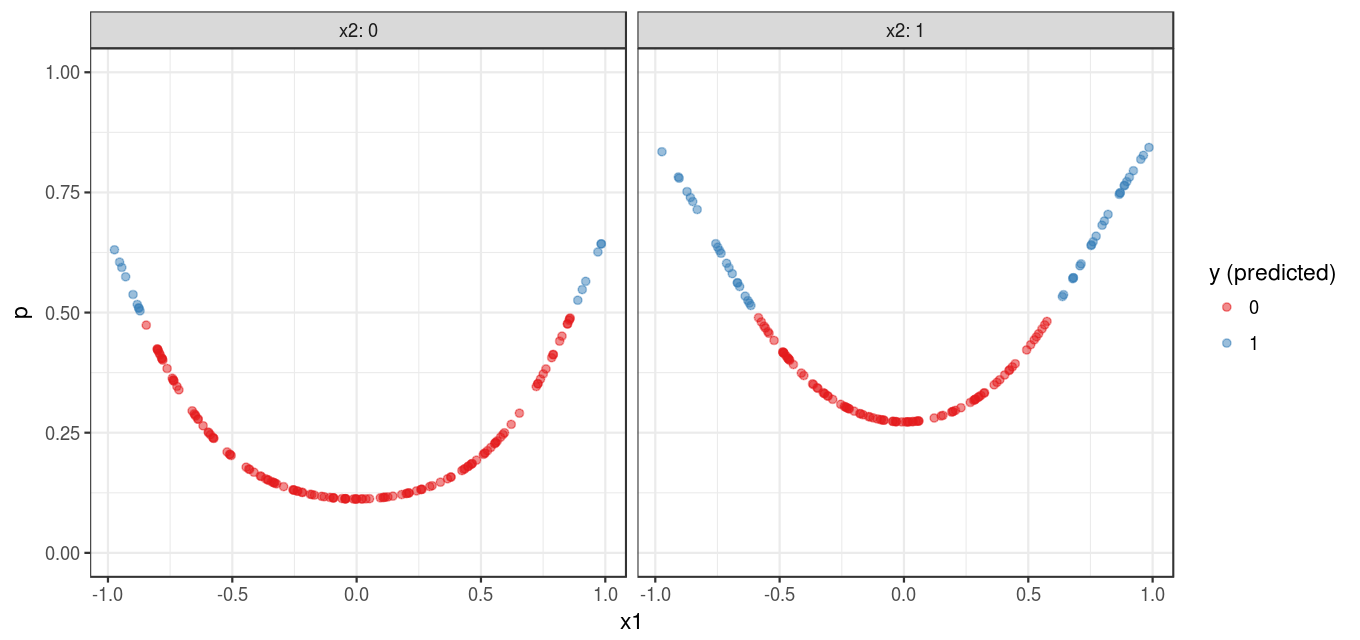
         y_predicted = if_else(p_predicted > 0.5, 1L, 0L))

Figure 2 shows the predicted probability of the outcome for each observation in the data set. The pattern shown in Figure 2 is comparable to that shown in Figure 1 .

Figure 2: Predicted probability

The following code shows the training error of the model:

mean(dat$y != dat$y_predicted)

#> [1] 0.2733333

An unexpected discovery

Logistic regression is a parametric method, so at first I expected the experiment results would have low variance³ (see my other post on the topic) even with a small sample size. But it didn’t turn out that way. To put the issue in a comparable context, assume \(g(p(X))\) from formula (3) is the continuous outcome to be predicted, a linear regression model would need a much smaller sample size to get robust estimates of the coefficients in \(X\).

³ You can run the code with different random seeds to see how the estimates of the coefficients change every time.

To be fair, the variance was not caused by the logistic regression algorithm itself; rather, it originated from the nature of classification problems. Given the right predictors and assumptions, the uncertainty of a continuous outcome is only affected by random noise. However, the same cannot be said for a categorical outcome. Even without random noise, the outcome is still uncertain unless the probability of the outcome is 1 or 0, which is rarely the case. Therefore, it is very likely that a small data set does not reflect the underlying assumption due to variance caused by the uncertainty. In addition, even if a good model that is consistent with the truth is built (like the one shown in the experiment), misclassification error rate may still be high due to the aforementioned uncertainty. With this in mind, sometimes it may be more preferable to use other metrics (predicted probability, sensitivity, specificity, etc.) instead of misclassification error to evaluate the performance of classification models.

Figure 1: Simulated data Figure 2: Predicted probability