A Brief Introduction to Bagged Trees, Random Forest and Their Applications in R

Abstract

Explains bagged trees and random forest in a nutshell.

Introduction

Continuing the topic of decision trees (including regression tree and classification tree), this post introduces the theoretical foundations of bagged trees and random forest, as well as their applications in R.

Bootstrap Aggregation and Bagged Trees

Bootstrap aggregation (i.e., bagging) is a general technique that combines bootstraping and any regression/classification algorithm to construct an ensemble. The process of bagging a model is very simple:

1. Generate \(k\) bootstrap samples of the original data.
2. Train the model on each of the samples.
3. For a new observation, each model provides a prediction and the \(k\) predictions are then averaged to give the final prediction.

Since the models in an ensemble are identically distributed (i.e., i.d.), the expectation of the average of the \(k\) predictions is the same as that of any individual prediction, meaning that the bias of the ensemble is the same as that of a single tree. The mechanism in which bagging improves model performance is reducing variance¹ (see my other post that explains the bias-variance tradeoff). Therefore, bagging is especially effective for models with low bias but high variance. Since decision trees are noisy but have relatively low bias, they can benefit a lot from bagging. Such an ensemble is called bagged trees.

¹ This is in contrast to boosting, which is an ensemble technique that aims at reducing bias.

The number of trees (i.e., \(k\)) is a hyperparameter for bagged trees. Generally speaking, the bigger the number of trees, the less the variance and hence the better performance of the ensemble. However, the most performance gain is typically achieved with the first 10 bootstrap samples. For some models with high variance (e.g., decision trees), performance gain is apparent up to about 20 bootstrap samples, and then tails off with very limited improvement beyond that point. It is usually pointless to construct an ensemble with more than 50 bootstrap samples, since the marginal performance gain is not worth the extra computational costs and memory requirements.

Random Forest

It should be noted that although the bagged trees are identically distributed, they are not necessarily independent. Since the bootstrap samples used to train each individual tree come from the same data set, it is not surprising that the trees may share some similar structure. This similarity, known as tree correlation, is an essential factor that prevents further reduction of variance (hence further improvement of performance) for bagged trees.

Tree correlation can be reduced by adding randomness to the process of tree construction; and if the amount of randomness is appropriate, the overall performance of an ensemble can be further improved. Random forest is such a modification of bagged trees that adopts this strategy. The independence among the trees makes random forest robust to a noisy outcome; however it may also underfit data when a outcome is not so noisy. The process of constructing a random forest is as follows:

1. Draw \(k\) bootstrap samples from the training set.
2. For each sample, grow an unpruned tree that only considers \(m_{try}\) predictors (which is a subset of all available predictors) at random for each split.
3. Output the ensemble of the trees.

To make a prediction for an observation: a random forest for regression averages the predictions given by the individual trees and returns the result; a random forest for classification chooses the majority class predicted by the individual trees.

There are two major hyperparameters for random forest, including:

1. The number of predicotrs (i.e., \(m_{try}\)) to consider at each split of a tree. \(m_{try}\) defaults to \(\frac{P}{3}\) for regression and \(\sqrt{P}\) for classification, where \(P\) is the total number of predictors. According to Kuhn and Johnson (2013), this hyperparameter does not have a drastic effect on the performance. Since random forest is computationally intensive, they suggested practitioners start with 5 values of \(m_{try}\) that are somewhat evenly spaced across the range of 2 and \(P\).
2. The number of trees (i.e., \(k\)) in the forest. Random forest is protected from over-fitting, therefore the performance of the forest improves monotonically as \(k\) increases. However, a bigger forest also demands more time and memory to train. As a starting point, Kuhn and Johnson (2013) suggested using at least 1000 trees, and then incorporate more trees until performance levels off. Note, however, that sometimes it may not require that many trees; for example Hastie, Tibshirani, and Friedman (2009) reported a case where 200 trees were sufficient.

Technically, there are other parameters that controls the tree construction process, such as those for decision trees. The defaults for these parameters in a random forest allow the trees to grow sufficiently deep so as to achieve low bias². Generally. there is no need to tune these parameters.

² The minimum number of observations in the terminal nodes of regression trees is 5, and that of classification trees is 1.

Fitting Bagged Trees and Random Forest in R

Here I will use random forest and bagged trees to build some regression models. The process of building classification models using the same algorithms are very similar; just store the outcome variable as a factor and it will be taken care of.

The following code generates a simulated data set on which the regression models will be trained:

library(tidyverse)
library(caret)
set.seed(1)
sample_size <- 300
dat <- tibble(
  x1 = runif(sample_size, min = -1, max = 1),
  x2 = sample(c(0L, 1L), sample_size, replace = T),
  x3 = sample(c(-1L, 0L, 1L), sample_size, replace = T),
  e = rnorm(sample_size, sd = 0.1),
  y = -2 + 3 * x1^2 + x2 + 2 * x3 + e
) %>%
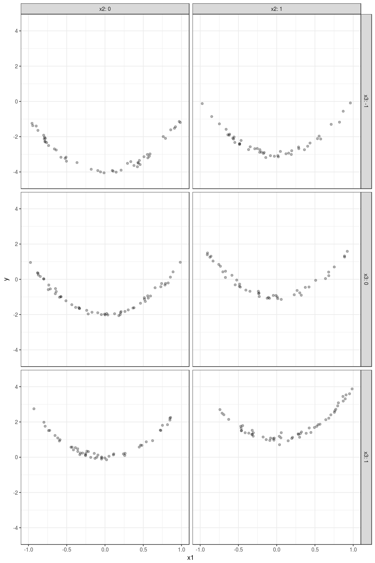
  mutate_at(vars(x2, x3), funs(as.factor(.)))

Figure 1 visualizes the simulated data set:

Figure 1: Simulated data

Here I use the caret::train() function to build the models and perform cross-validation. Note that bagged tree can be seen as a special case of random forest, where the number of predictors to consider for each split of a tree (i.e., mtry) equals the number of all available predictors. Therefore, in this example, when mtry = 4 (note that x3 is expanded to two dummy variables, so the total number of predictors is 4 instead of 3), a bagged ensemble of trees is built. To save computational time, the number of trees ntree is set to 50³. The importance parameter should be set to T if variable importance measure are to be calculated.

³ In this example, the performance of the forest will not be drastically improved with more than 50 trees.

fit_rf <- train(y ~ x1 + x2 + x3, data = dat, method = "rf", importance =  T,
                tuneGrid = expand.grid(mtry = 2:4),
                ntree = 50,
                trControl = trainControl(method = "cv"))

fit_rf

#> Random Forest 
#> 
#> 300 samples
#>   3 predictors
#> 
#> No pre-processing
#> Resampling: Cross-Validated (10 fold) 
#> Summary of sample sizes: 269, 269, 271, 268, 272, 269, ... 
#> Resampling results across tuning parameters:
#> 
#>   mtry  RMSE       Rsquared   MAE      
#>   2     0.4490445  0.9522216  0.3558190
#>   3     0.2736851  0.9793394  0.2047065
#>   4     0.2299081  0.9840169  0.1642898
#> 
#> RMSE was used to select the optimal model using the smallest value.
#> The final value used for the model was mtry = 4.

The result shows that the \(mtry\) parameter for the best model is 4, which means the bagged trees out-performs random forest in this case. The predictions can be obtained with the predict() function.

dat <- dat %>%
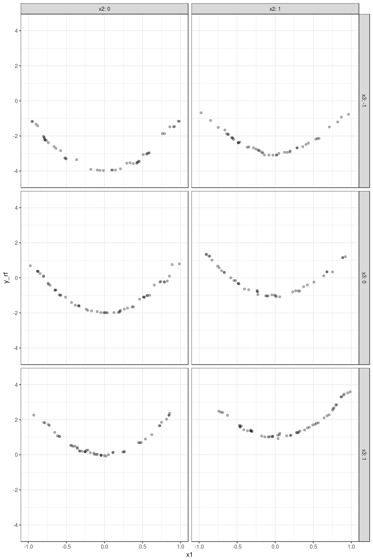
  mutate(y_rf = predict(fit_rf, type = "raw"))

Figure 2 shows the predictions. Compared with Figure 1 , it is easy to see that the model almost perfectly captures the variation of the data⁴.

⁴ If a CART regression tree is trained on the data with minsplit = 10 and minbucket = 5 (which are the defaults of a singe tree in a random forest), you can see that the predictions are less granular than those given by the ensemble.

Figure 2: Predictions

Variable importance can be obtained with the varImp() function:

varImp(fit_rf)

#> rf variable importance
#> 
#>     Overall
#> x30  100.00
#> x31   71.77
#> x21   34.16
#> x1     0.00

References

Figure 1: Simulated data Figure 2: Predictions

References

Hastie, Trevor, Robert Tibshirani, and Jerome Friedman. 2009. The Elements of Statistical Learning: Data Mining, Inference, and Prediction. 2nd ed. New York: Springer.

Kuhn, Max, and Kjell Johnson. 2013. Applied Predictive Modeling. 1st ed. New York: Springer.