How to Plot ROC and Precision-Recall Curves
Introduction
Receiver Operator Characteristic (ROC) curves and Precision-Recall (PR) curves are commonly used to evaluate the performance of classifiers. However, literatures have indicated that there are many misconceptions and misuses of these methods in practice(Fawcett 2006; Pinker 2018). To avoid such pitfalls, it is necessary to understand ROC curves and PR curves thoroughly.
Explaining ROC curves and PR curves in depth is a very ambitious take which is unlikely to be achieved in one single post. Therefore, this post will serve as an opening for following posts by introducing how to plot ROC and PR curves. Additionally, since the area under these curves (AUC) is an important summary metric, its calculation will also be introduced. To be more concrete, this post will present an example with code to demonstrate implementation. The most essential functions come from the tidymodels package in R, which is a new member of the tidyverse family.
The definition of relevant concepts and metrics
Before diving in to plotting the curves, we need to define some concepts and metrics.
A binary classifier predicts each example as either positive or negative. Depending on whether the prediction is consistent with the truth, each example falls into one of four categories:
- true positive: a positive example that is correctly classified as positive;
- false positive: a negative example that is incorrectly classified as positive;
- true negative: a negative example that is correctly classified as negative;
- false negative: a positive example that is incorrectly classified as negative.
By counting the number of examples in each of the four categories, we can obtain a confusion matrix, like the one shown below:
| Table 1. Confusion matrix for binary classification problems | ||
|---|---|---|
| Prediction | Truth | |
| Positive | Negative | |
| Positive | a1 | b2 |
| Negative | c3 | d4 |
| 1 Number of true positives. 2 Number of false positives. 3 Number of false negatives. 4 Number of true negatives. | ||
With the numbers in the confusion matrix, we can define the metrics that will be used to plot ROC/PR curves, including: sensitivity, specificity, precision and recall (note that sensitivity and recall are the same):
\[ \begin{align} sensitivity &= \frac{a}{a + c} \\ specificity &= \frac{d}{b + d} \\ precision &= \frac{a}{a + b} \\ recall &= \frac{a}{a + c} \end{align} \quad (1) \]
By now, we have covered the most fundamental concepts and metrics that underlie ROC/PR curves. In brief, an ROC graph is a two-dimensional graph in which \(sensitivity\) is plotted on the vertical axis and \(1 - specificity\) is plotted on the horizontal axis; a PR curve is also a two-dimensional graphy, but with \(precision\) plotted on the vertical axis and \(recall\) plotted on the horizontal axis. However, there is one more thing we need to talk about before we can actually plot the curves.
Probabilistic score and threshold
Some classifiers, such as decision trees, are designed to produce only a class prediction. When such a discrete classifier is applied to a test set, it only yields a single confusion matrix and thus a single value for each of the aforementioned metrics. In such cases, an ROC/PR curve can not be plotted since there is just one point in the respective space.
Other classifiers, such as logistic regression, produce a probabilistic score that represents the degree to which an example is a member of a class. Such a probabilistic classifier can be used with a threshold to produce class predictions: if the score is greater than the threshold, the example is considered to be a positive, otherwise a negative. By varying the threshold, we can get multiple confusion matrices, each corresponding to a different point in the ROC space and the PR space. By connecting these points, we get the ROC and PR curves for the classifier.
In the remaining text, I will use the output of a probabilistic classifier as an example for demonstration. However, it should be noted that there are ways to obtain probabilistic scores as predictions from discrete classifiers so that ROC and PR curves can be plotted1.
1 For example, we can use the class proportions in the leaf nodes of a decision tree as such a score. Even for a classifier that does not contain any such internal statistics, we can still use bootstrap aggregating to generate an ensemble of the classifier, and then use the votes to compute one.
Computing the metrics
library(tidymodels)
theme_set(theme_bw())
Below is a dataframe named dat that contains 20 examples. The actual outcomes are store in the column named true_class with two possible values: positive and negative. The column named score stores the probability scores produced by the classifier. For the purpose of demonstration, I have order the rows by score in a descending order.
dat <- tibble(true_class = c("positive", "positive", "negative", "positive", "positive", "positive", "negative", "negative", "positive", "negative",
                        "positive", "negative", "positive", "negative", "negative", "negative", "positive", "negative", "positive", "negative"),
              score = c(0.9, 0.8, 0.7, 0.6, 0.55, 0.54, 0.53, 0.52, 0.51, 0.505,
0.4, 0.39, 0.38, 0.37, 0.36, 0.35, 0.34, 0.33, 0.30, 0.1))print(dat)## # A tibble: 20 x 2
## true_class score
## <chr> <dbl>
## 1 positive 0.9
## 2 positive 0.8
## 3 negative 0.7
## 4 positive 0.6
## 5 positive 0.55
## 6 positive 0.54
## 7 negative 0.53
## 8 negative 0.52
## 9 positive 0.51
## 10 negative 0.505
## 11 positive 0.4
## 12 negative 0.39
## 13 positive 0.38
## 14 negative 0.37
## 15 negative 0.36
## 16 negative 0.35
## 17 positive 0.34
## 18 negative 0.33
## 19 positive 0.3
## 20 negative 0.1First, let’s set the threshold for score using the highest value 0.92, and classify examples with \(score >= 0.9\) as positives and the others as negatives. We will store the class prediction in a column named pred_class:
2 I have simplified some descriptions here. As you will see in following text, the highest threshold for calculating sensitivity and specificity should be Inf, and the lowest one should be -Inf. Also, while the highest threshold for calculating precision and recall is still Inf, the lowest threshold is not.
dat <- dat %>%
  mutate(pred_class = if_else(score >= 0.9, "positive", "negative")) %>%
  mutate_at(vars(true_class, pred_class), list(. %>% factor() %>% forcats::fct_relevel("positive")))
Note that the following functions only accept factors as input, and by default the first level will be considered as the level of interest3. The latter behavior has an implication on how the metrics should be calculated. Therefore, it is necessary to convert the two columns into factors and set positive to be the first level (important: if you don’t pay attention to it, you may obtain the wrong results!).
3 You can change this behavior with a function parameter called event_level; see the function documentation for more details.
Then we can use the sens() function to calculate sensitivity, using the columns true_class and pred_class:
dat %>%
  sens(true_class, pred_class)
## # A tibble: 1 x 3
## .metric .estimator .estimate
## <chr> <chr> <dbl>
## 1 sens binary 0.1The result shows that the sensitivity of the classifier with 0.9 as the score threshold is 0.1. To calculate specificity, precision and recall, use spec(), precision() and recall() respectively; the usage is the same.
Next, let’s lower the threshold and set it to the second highest value of score (i.e., 0.8), and repeat the same procedure above. By doing this, we get another set of sensitivity, specificity, precision and recall. If we keep lowering the threshold until we reach the bottom, we will eventually obtain a full range of values for the metrics, which can be used to plot the curves.
Repeating the above procedure for each threshold is cumbersome, but fortunately, there are two functions that handles everything: roc_curve() and pr_curve(). Just pass the true_class and score columns as inputs to these functions, and you’ll get the results. The following code shows how:
roc_dat <- dat %>%
  roc_curve(true_class, score)

roc_dat
## # A tibble: 22 x 3
## .threshold specificity sensitivity
## <dbl> <dbl> <dbl>
## 1 -Inf 0 1
## 2 0.1 0 1
## 3 0.3 0.1 1
## 4 0.33 0.1 0.9
## 5 0.34 0.2 0.9
## 6 0.35 0.2 0.8
## 7 0.36 0.3 0.8
## 8 0.37 0.4 0.8
## 9 0.38 0.5 0.8
## 10 0.39 0.5 0.7
## # … with 12 more rowspr_dat <- dat %>%
pr_curve(true_class, score)
pr_dat## # A tibble: 21 x 3
## .threshold recall precision
## <dbl> <dbl> <dbl>
## 1 Inf 0 NA
## 2 0.9 0.1 1
## 3 0.8 0.2 1
## 4 0.7 0.2 0.667
## 5 0.6 0.3 0.75
## 6 0.55 0.4 0.8
## 7 0.54 0.5 0.833
## 8 0.53 0.5 0.714
## 9 0.52 0.5 0.625
## 10 0.51 0.6 0.667
## # … with 11 more rowsPlotting the curves
Each row in roc_dat represents a point in the ROC space. To plot the ROC curve, we first order the rows by the column .threshold (either in a descending or ascending order), and then connect the points in that order. The following code shows how:
roc_dat %>%
  arrange(.threshold) %>% # this step is not strictly necessary here because the rows are already ordered by `.threshold`
  ggplot() +
  geom_path(aes(1 - specificity, sensitivity)) + # connect the points in the order in which they appear in the data to form a curve
  geom_abline(intercept = 0, slope = 1, linetype = "dotted") + # add a reference line by convention
  coord_equal()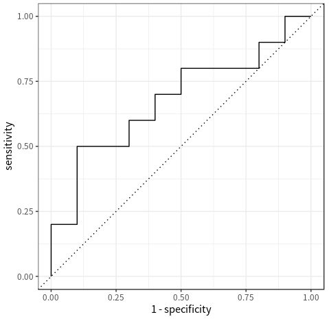
The process of plotting the PR curve is very similar:
pr_dat %>%
  arrange(.threshold) %>% # this step is not strictly necessary here because the rows are already ordered by `.threshold`
  ggplot() +
  geom_path(aes(recall, precision)) + # connect the points in the order in which they appear in the data to form a curve
  coord_equal()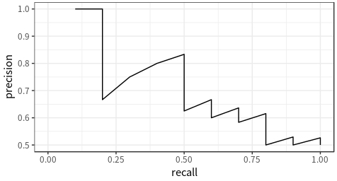
The code above shows how to plot the curves using native ggplot2 functions. If you don’t feel like writing extra code, there is also a handy function called autoplot() that accepts the output of roc_curve() or pr_curve() and plots the curves correspondingly.
Calculating area under curve
Both ROC curve and PR curve are two-dimensional depictions of classifier performance. In some cases when the curves of multiple classifiers intersect, it is hard to tell which one is superior. Therefore, it is preferrable to extract a single scalar metric from these curves to compare classifiers. The most common method is to calculate the area under an ROC curve or a PR curve, and use that area as the scalar metric.
To calculate the area under an ROC curve, use the roc_auc() function and pass the true_class and the score columns as inputs:
dat %>%
  roc_auc(true_class, score)
# A tibble: 1 x 3
.metric .estimator .estimate
<chr> <chr> <dbl>
1 roc_auc binary 0.68To calculate the area under an ROC curve, use the pr_auc() function and pass the same columns as inputs:
dat %>%
  pr_auc(true_class, score)
# A tibble: 1 x 3
.metric .estimator .estimate
<chr> <chr> <dbl>
1 pr_auc binary 0.619Summary
This post introduces the metrics required to plot ROC/PR curves, how to compute these metrics and plot the curves using R. However, it has not covered how to interpret the curves, or how to use them in practice (e.g., model selection/tuning), etc. These will be the topics of a few following posts.