A Brief Introduction to Various Correlation Coefficients and When to Use Which
Introduction
Correlation coefficients are used to measure how strong a relationship is between two (and in some cases more) variables. There are various kinds of coefficients, and sometimes it can be difficult to decide when to use which.
This post serves to introduce several frequently used correlation coefficients including Pearson’s \(r_p\), Spearman’s \(r_s\), Kendall’s \(\tau\) and Cramer’s \(v\). These coefficients can be used to calculate the correlation between variables measured at ratio, interval, ordinal or nominal scales (Wikipedia 2019b). For each of these coefficients, the underlying assumptions, definition, interpretation, as well as application in R will be presented.
The code provided in this post requires the following packages:
library(tidyverse)
library(DescTools)
Pearson’s \(r_p\)
Pearson’s \(r_p\) was developed by Karl Pearson about a decade after Francis Galton completed the theory of bivariate correlation in 1885 (Wikipedia 2019c). It is a parametric measure of linear correlation between two variables; to use it, the following assumptions must hold (Laerd Statistics 2019c):
- The variables are of either interval or ratio scale.
- The variables are approximately normally distributed.
- There is a linear relationship between the two variables.
- Outliers are either removed entirely or are kept to a minimum.
- There is homoscedasticity of the data.
Let \((X, Y)\), i.e., \((x_1, y_1), (x_2, y_2), ..., (x_n, y_n)\), denote the pair of variables between which the correlation will be calculated, then \(r_p\) can be defined as the covariance of the two variables divided by the product of their standard deviations:
\[ \begin{align} r_p(X, Y) &= \frac{\frac{\sum_{i=1}^n(x_i - \bar{x})(y_i - \bar{y})}{n - 1}}{\sqrt{\frac{\sum_{i=1}^{n}(x_i - \bar{x})^2}{n - 1} \frac{\sum_{i=1}^{n}(y_i - \bar{y})^2}{n - 1}}} \\ &= \frac{\sum_{i=1}^n(x_i - \bar{x})(y_i - \bar{y})}{\sqrt{\sum_{i=1}^{n}(x_i - \bar{x})^2 \sum_{i=1}^{n}(y_i - \bar{y})^2}} \end{align} \quad (1) \]
Pearson’s correlation coefficient \(r_p\) ranges from −1 to 1. A value of 0 implies no linear association between the two variables. A positive value implies a positive association between the two variables (i.e., as the value of one variable increases, the value of the other variable also increases). A negative value implies a negative (i.e., as the value of one variable increases, the value of the other variable decreases). Specifically, a value of 1 or -1 implies a perfect linear association with all the points lying exactly on a line. I refer interested readers to an article that discusses the interpretations of \(r_s\) in more details (Rodgers and Nicewander 1988).
The stats::cor() function with method = "pearson" (which is the default) provides an implementation of \(r_p\) in R. See the next section for a demonstration.
Spearman’s \(r_s\)
Spearman’s \(r_s\) was developed by Charles Spearman at around 1904 to measure the monotonic correlation between two variables (Wikipedia 2019d). Although Spearman’s \(r_s\) is a nonparametric measure, there are still some conditions for its applicability (Laerd Statistics 2019d):
- The variables are of either interval or ratio scale.
- There is a monotonic relationship between the two variables.
- Outliers are kept to a minimum.
The Spearman’s correlation coefficient \(r_s\) between two variables is equal to the Pearson correlation between the rank values of those two variables. Therefore, by changing the values of the variables to their ranks respectively, \(r_s\) can also be calculated using equation (1).
Spearman’s correlation coefficient \(r_s\) also ranges from −1 to 1. Its interpretation is very much like that of Pearson’s \(r_p\) except that Spearman’s \(r_s\) measures how well the relationship between two variables can be described using a monotonic function, which includes but is not limited to linearity.
In R, \(r_s\) can be calculated using the stats::cor() function with method = "spearman"; see below for an example.
It is useful to note that, as long as the relationship between two variables are monotonic, \(r_s\) will always return a value of 1 or -1; however, for \(r_p\) to return a value of 1 or -1, the relationship has to be not only monotonic, but also linear. The following code demonstrates this fact (note that in both cases, \(r_s\) return 1, while \(r_p\) only returns 1 in one cases):
set.seed(1)
dat_linear <- tibble(x = runif(20, min = -1, max = 1)) %>%
  mutate(y = x, f = "y = x")

dat_cubic <- tibble(x = runif(20, min = -1, max = 1)) %>%
  mutate(y = x^3, f = "y = x^3")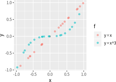
cor(dat_linear$x, dat_linear$y, method = "pearson")# 1.00cor(dat_cubic$x, dat_cubic$y, method = "pearson")# 0.90cor(dat_linear$x, dat_linear$y, method = "spearman")# 1.00cor(dat_cubic$x, dat_cubic$y, method = "spearman")# 1.00It is also useful to note that Spearman’s \(r_s\) does not account for the number of ties in the data and may therefore underestimate the correlation when there are many ties. For this reason, it is inappropriate to use Spearman’s \(r_s\) to measure the correlation between ordinal variables, which typically contain many ties (Kendall 1945).
Kendall’s \(\tau\)
The Kendall’s \(\tau\) coefficient was first proposed by Kendall (1938). This original coefficient is known as \(\tau_a\) and it has the following conditions for applicability (Laerd Statistics 2019b):
- The variables are of either interval, ratio or ordinal scale.
- There is a monotonic relationship between the two variables.
Let \((X, Y)\), i.e., \((x_1, y_1), (x_2, y_2), ..., (x_n, y_n)\), denote the pair of variables between which the correlation will be calculated. For any pair of observations \((x_i, y_i)\) and \((x_j, y_j)\) where \(i < j\), it is said to be concordant either if \(x_i > x_j\) and \(y_i > y_j\), or if \(x_i < x_j\) and \(y_i < y_j\); conversely, it is said to be disconcordant either if \(x_i > x_j\) and \(y_i < y_j\), or if \(x_i < x_j\) and \(y_i > y_j\). If \(x_i = x_j\) or \(y_i = y_j\), the pair is called a tie and is neither concordant or disconcordant. If we denote the number of concordant pairs, disconcordant pairs, and all pairs respectively as \(n_c\) \(n_d\) and \(n_0\)1, then \(\tau_a\) can be defined as:
1 To be more concrete, \(n_0 = \frac{n(n - 1)}{2}\), where \(n\) denotes the number of observations in the data.
\[ \tau_a = \frac{n_c - n_d}{n_0} \quad (2) \]
Notice that \(\tau_a\) does not account for the number of ties in the data and therefore may be biased. For this reason, Kendall proposed a revised coefficient, known as \(\tau_b\), to make adjustments for ties(Kendall 1945). The \(\tau_b\) coefficient is defined as:
\[ \tau_b = \frac{n_c - n_d}{\sqrt{(n_0 - n_1)(n_0 - n_2)}} \quad (3) \]
where \(n_1\) and \(n_2\) represents the number of all pairs that contain ties of the first and second variable, respectively2.
2 To be more concrete, \(n_1 = \frac{\sum_{i}t_i(t_i - 1)}{2}\), \(n_2 = \frac{\sum_{j}u_j(u_j - 1)}{2}\), where \(t_i\)/\(u_j\) denotes the number of tied values in the \(i^{th}\)/\(j^{th}\) group of ties for the first/second variable, respectively
When applied to ordinal variables, \(\tau_b\) assumes that the two variables forms a square \(r \times c\) (\(r = c\)) contingency table (i.e., they have the same number of unique values), otherwise the coefficient can not attain \(\pm 1\). To extent the coefficient to deal with data based on non-square \(r \times c\) (\(r \neq c\)) contingency tables, Stuart proposed a variant known as \(\tau_c\) (Stuart 1953). It is defined as:
\[ \tau_c = \frac{2(n_c - n_d)}{n^2 \frac{(m - 1)}{m}} \quad (4) \]
where \(n\) is the number of observations and \(m = min(r, c)\).
\(\tau_a\), \(\tau_b\) and \(\tau_c\) range from -1 to 1, with positive values indicating positive associations and negative values indicating negative associations.
\(\tau_b\)3 and \(\tau_c\) can be calculated using DescTools::KendallTauB() and DescTools::StuartTauC(), respectively. To demonstrate the differences, consider the contingency table given below:
3 \(\tau_b\) can also be calculated using stats::cor() with method = "kendall".
dat_ordinal <- matrix(c(5, 5, 0, 0, 0, 0,
                        0, 0, 5, 5, 0, 0,
                        0, 0, 0, 0, 5, 5),
                      byrow = T, ncol = 6,
                      dimnames = list(c("a", "b", "c"),
                                      c("A1", "A2", "B1", "B2", "C1", "C2"))) %>%
  as.table() %>%
  as.data.frame() %>%
  group_split(Var1, Var2) %>%
  map_dfr(function(x) {
    rep(list(x), times = x$Freq) %>%
      bind_rows()
  }) %>%
  transmute_at(vars(Var1, Var2),
               ~ forcats::fct_inorder(., ordered = T))

table(dat_ordinal$Var1, dat_ordinal$Var2)
## A1 A2 B1 B2 C1 C2
## a 5 5 0 0 0 0
## b 0 0 5 5 0 0
## c 0 0 0 0 5 5When we calculate the correlation using different coefficients, we can see the difference:
KendallTauB(dat_ordinal$Var1, dat_ordinal$Var2)# 0.89StuartTauC(dat_ordinal$Var1, dat_ordinal$Var2)# 1.00The results shows that when the table is rectangular, \(\tau_c\) can still attain a value of 1, while \(\tau_b\) can not.
It is useful to note that while \(r_s\) and \(\tau\) (all variants) can be used to measure the correlation between ratio or interval variables, Croux and Dehon (2010)’s study shows that \(\tau\) is more robust and slightly more efficient than \(r_s\). However, \(\tau\) takes a longer time to compute; this is quite perceptible when the sample size reaches 10000.
Cramer’s \(v\)
Cramer’s \(v\) was developed by Cramér (1999) to measure the association between two categorical variables. Since Cramer’s \(v\) is based on Chi-squared test, they share similar assumptions (Laerd Statistics 2019a):
- The variables should be measured at an ordinal or nominal level.
- Each variable should contain two or more independent groups.
Cramer’s \(v\) is defined as:
\[ v = \sqrt{\frac{\chi^2 / n}{min(r - 1, c - 1)}} \quad (5) \]
where \(\chi^2\) denotes Pearson’s chi-squared statistic4, \(n\) denotes the sample size, \(r\) and \(c\) respectively denotes the number of rows and columns in the contingency table of the two variables. Note that when \(r = c = 2\), Cramer’s \(v\) is equivalent to the Phi coefficient \(\phi\), which is intended for binary correlation (Wikipedia 2018).
4 The calculation of \(\chi^2\) can be found in (Wikipedia 2019a).
Unlike the other coefficients, Cramer’s \(v\) ranges from 0 to 1, with 0 indicating no association at all and 1 indicating perfect association.
Cramer’s \(v\) can be calculated using DescTools::CramerV(); for example:
set.seed(1)
dat_nominal <- tibble(Var1 = sample(letters[1:3], 10000, replace = T),
                      Var2 = sample(letters[1:5], 10000, replace = T))

CramerV(dat_nominal$Var1, dat_nominal$Var2)
# 0.02Since the data are generated randomly, the correlation is very close to 0.
Note that although Cramer’s \(v\) can be applied to ordinal variables, there will loss of information since the coefficient does not care about the order of the categories. In such cases, it is more appropriate to use Kendall’s \(\tau\) coefficients.
Some notes on interpreting the magnitude of a correlation
There are many different guidelines for interpreting the magnitude of a correlation (Maher et al. 2013; Mukaka 2012; Hemphill 2003). While there are quite some differences, most would agree that a correlation coeffcient between -0.1 and 0.1 indicates negligible association, and a coefficient greater than 0.9 or less than -0.9 indicates an extremely strong association. However, these thresholds are quite arbitrary and should be used with caution. Two coeffients with the same value but are calculated using different methods do not necessarily indicate the same level of association. Moreover, under different contexts, the interpretations of the coefficients calculated using the same method can also differ. For example, a correlation of 0.8 may be very low if one is verifying a physical law using high-quality instruments, but may be regarded as very high in social or medical sciences where there may be a greater contribution from complicating factors (Wikipedia 2019c).
Conclusions
To summarise, here are some key take-aways on deciding when to use which method to measure correlation:
- If the two variables satisfy the assumptions of Pearson’s \(r_p\), then \(r_p\) would be the obvious choice due to its parametric nature, which brings more statistical efficiency(Croux and Dehon 2010).
- If the two variables are of ratio or interval scale, but do not satisfy other assumptions of Pearson’s \(r_p\), then:
- use Kendall’s \(\tau_b\) (which is directly available from base R) when the sample size is small (\(n \leq 10000\)) and significant outliers are found in the data.
- use Spearman’s \(r_s\) when the sample size is large (\(n > 10000\)), or when no significant outliers are found in the data.
- If the two variables are of ordinal scale, then:
- use \(\tau_b\) when the contingency table is square (\(\tau_c\) is also appropriate, but it is not as conventient since you need to install additional packages in R);
- use \(\tau_c\) when the contingency table is rectangular.
- If the two variables are of nominal scale, then use Cramer’s \(v\).
- If the two variables are of binary scale, then use Phi coefficient \(\phi\). Recall that \(\phi\) is a special case of Cramer’s \(v\) when \(r = c = 2\). Also note that when a Pearson correlation coefficient estimated for two binary variables will return the Phi coefficient (Wikipedia 2018). This means that you can either use the formula for Pearson’s \(r_p\) or Cramer’s \(v\) to calculate \(\phi\).
For those curious, Baak et al. (2018) recently proposed a new correlation coefficient that covers many types of variables (nominal, ordinal, interval) and has some nice characteristics. It seems like a alternative to the classic methods mentioned in this post. However, it also seems more complicated and therefore harder to interpret.