RetinaNet Explained and Demystified
Introduction
Recently I have been doing some research on object detection, trying to find a state-of-the-art detector for a project. I found several popular detectors including: OverFeat (Sermanet et al. 2013), R-CNN (Girshick et al. 2013), Fast R-CNN (Girshick 2015), SSD (Liu et al. 2016), R-FCN (Dai et al. 2016), YOLO (Redmon et al. 2016), Faster R-CNN (Ren et al. 2017) and RetinaNet (Lin, Goyal, et al. 2017). According to the paper, RetinaNet showed both ideal accuracy and speed compared to other detectors while still keeping a very simple construct; plus, there is an opensource implementaion by Gaiser et al. (2018). Therefore, RetinaNet appears to be an ideal candidate for the project. To use the detector appropriately, I need to study its design and intuitions. Therefore, I read the original paper and many related ones carefully and post shares what I have learnt.
Note: for a brief introduction and comparison among popular detectors before RetinaNet (e.g., R-CNN), see (Tryolabs 2017; Xu 2017); I have also found a post by Hollemans (2018) to be very informative.
Update: here is another related post.
RetinaNet decomposed
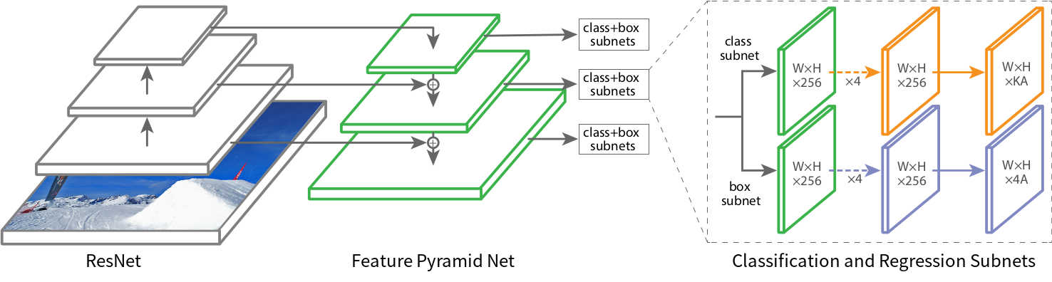
In essence, RetinaNet is a composite nework composed of:
- a backbone network called Feature Pyramid Net, which is built on top of ResNet and is responisble for computing convolutional feature maps of an entire image;
- a subnetwork responsible for performing object classification using the backbone’s output;
- a subnetwork responsible for performing bounding box regression using the backbone’s output.
Figure 1 gives a visualization of the construction.
The backbone network
RetinaNet adopts the Feature Pyramid Network (FPN) proposed by Lin, Dollar, et al. (2017) as its backbone, which is in turn built on top of ResNet (ResNet-50, ResNet-101 or ResNet-152)1 in a fully convolutional fashion. The fully convolutional nature enables the network to take an image of an arbitrary size and outputs proportionally sized feature maps at multiple levels in the feature pyramid.
1 Note that FPN is actually independent of the underlying convolutional network architecture, which means other architecures may also be used to build FPN. However, following the original paper, this post will focus on the implementation using ResNet.
The construction of FPN involves two pathways which are connected with lateral connections. They are described as below.
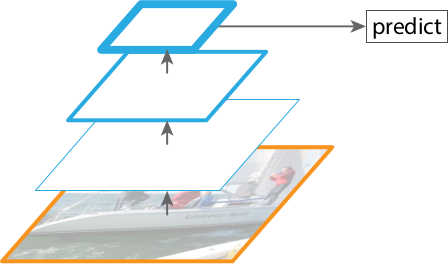
Bottom-up pathway. Recall that in ResNet, some consecutive layers may output feature maps of the same scale; but generally, feature maps of deeper layers have smaller scales/resolutions. The bottom-up pathway of building FPN is accomplished by choosing the last feature map of each group of consecutive layers2 that output feature maps of the same scale. These chosen feature maps will be used as the foundation of the feature pyramid. The bottom-up pathway is visualized in Figure 2 .
2 In the original paper, these layers are said to be in the same network stage.
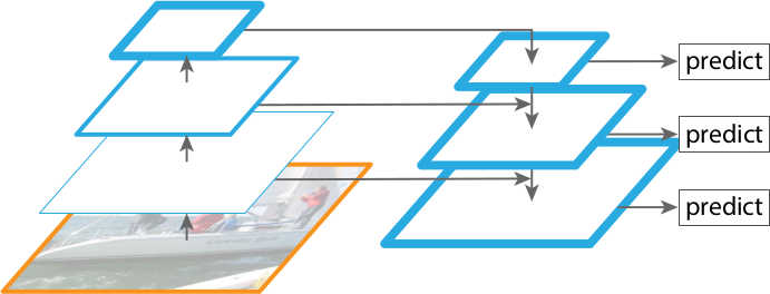
Top-down pathway and lateral connections. Using nearest neighbor upsampling, the last feature map from the bottom-up pathway is expanded to the same scale as the second-to-last feature map. These two feature maps are then merged3 by element-wise addition to form a new feature map. This process is iterated until each feature map from the bottom-up pathway has a corresponding new feature map connected with lateral connections. The top-down pathway and lateral connections are visualized in Figure 3 .
3 The feature map directly taken from the bottom-up pathway also undergoes a \(1 \times 1\) convolution to reduce channel dimensions before the merge.
There are altogether five levels in the pyramid (the figures only shows three) denoted as \(P_3, ..., P_7\), where \(P_l\) has resolution \(2^l\) lower than the input. The intuition behind FPN are described as below.
In real-world object detection, objects from the same class may be presented in a wide range of scales in images. This leads to some decrease in detection accuracy, especially for small objects. This is because feature maps from higher levels of the pyramid are spatially coarser, though semantically stronger. Therefore, only using the last feature map of a network to make the prediction (see Figure 2 ) is less ideal.
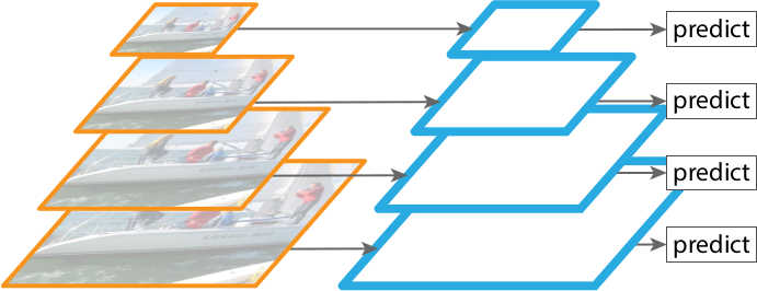
One solution would be to generate different scales of an image and feed them to the network separately for prediction ( Figure 4 ). This approach is termed “feature pyramids built upon image pyramids” and was widely adopted before the era of deep learning. However, since each image needs to be fed into the network multiple times, this approach also introduces a significant increase in test time, making it impractical for real-time applications.
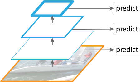
Another solution would be to simply use multiple feature maps generated by a ConvNet for prediction ( Figure 5 ), and each feature map would be used to detect objects of different scales. This is an approach adopted by some detectors like SSD. However, although the approach requires little extra cost in computation, it is still sub-optimal since the lower feature maps cannot sufficiently obtain semantic features from the higher ones.
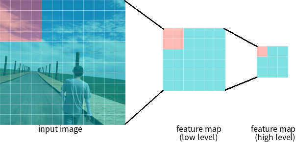
Finally, we turn to FPN. As mentioned, FPN is built in a fully convolutional fashion which can take an image of an arbitrary size and output proportionally sized feature maps at multiple levels. Higher level feature maps contain grid cells that cover larger regions of the image and is therefore more suitable for detecting larger objects; on the contrary, grid cells from lower level feature maps are better at detecting smaller objects (see Figure 6 4). With the help of the top-down pathway and lateral connections, which do not require much extra computation, every level of the resulting feature maps can be both semantically and spatially strong. These feature maps can be used independently to make predictions and thus contributes to a model that is scale-invariant and can provide better performance both in terms of speed and accuracy.
4 There are 256 channels in each feature map, but for simplicity they are not drawn in the figure.
Classification subnet
The classification subnet is a fully convolutional network (FCN) attached to each FPN level. The subnet consists of four \(3 \times 3\) convolutional layers with 256 filters, followed by RELU activations. Then, another \(3 \times 3\) convolutional layer with \(K \times A\) filters are applied, followed by sigmoid activation (instead of softmax activation)5. The subnet has shared parameters across all levels. The shape of the output feature map would be \((W, H, KA)\), where \(W\) and \(H\) are proportional to the width and height of the input feature map, \(K\) and \(A\) are the numbers of object class and anchor box (see Figure 1 ), which I’ll explain later.
5 According to the paper, this leads to greater numerical stability when computing the loss.
Regression subnet
The regression subnet is attached to each feature map of the FPN in parallel to the classification subnet. The design of the regression subnet is identical to that of the classification subnet, except that the last convolutional layer is \(3 \times 3\) with \(4A\) filters. Therefore, the shape of the output feature map would be \((W, H, 4A)\)6.
6 Note that unlike many previous detectors (R-CNN, Fast R-CNN, etc.), the RetinaNet’s bounding box regressor is class-agnostic, which leads to fewer parameters but is also equally effective.
A closer look at the subnets
Both the classification subnet and the regression subnet have output feature maps with width \(W\) and height \(H\). As mentioned, each of the \(W \times H\) slices corresponds to a region in the input image (similar to what is shown in Figure 6 ); but what about the channels? Why does the classification subnet outputs \(KA\) channels while the regression subnet outputs \(4A\) channels, and what do these channels respectively correspond to? To answer these questions, we first need to introduce a concept called anchor box, which was first proposed by Ren et al. (2017).
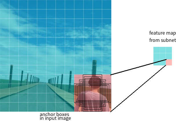
Let’s suppose that, given an input image, the width and height of a feature map output by the FPN is \(3 \times 3\). Then for each one of these nine grid cells, the RetinaNet defines \(A = 9\) boxes called anchor boxes, each having different sizes and aspect ratios and covering an area in the input image ( Figure 7 )7. Each anchor box is responsible for detecting the existence of objects from \(K\) classes in the area that it covers. Therefore, each anchor box corresponds to \(K\) numbers indicating the class probabilities. And since there are \(A\) bounding boxes per grid, the output feature map of the classification subnet has \(KA\) channels.
7 Note that although anchors are defined based on the feature map, the final anchors reference the original image.
In addition to detecting the existence/class of objects, each anchor box is also responsible for detecting the size/shape of objects (if any). This is done through the regression subnetwork, which outputs 4 numbers for each anchor box that predict the relative offset (in terms of center coordinates, width and height) between the anchor box and the ground truth box. Therefore, the output feature map of the regression subnet has \(4A\) channels.
By now, we can see that the subnets actually generates many numbers (\(K\) from the classification subnet, \(4\) from the regression subnet) for a large number (\(\sum_{l=3}^{7}{W_l \times H_l}\); where \(l\) denotes the level of pyramid; \(W\) and \(H\) are the width and height of the output feature map of the subnet.) of anchor boxes. Using these numbers to refine the anchor boxes, we get bounding box predictions. To calculate the loss for training, we need to compare the predictions with the ground-truths. However, how do we determine which bounding box should be compared with which ground-truth box, and what loss functions should be used?
Matching predictions with ground-truths
Note that the predictions output by the subnets are stored in output tensors. To calculate the loss, we would also need to create target tensors, each with the same shape as its corresponding output tensor and fill them with ground-truth labels at matching positions.
Also note that the match is actually performed between each anchor box and a ground-truth box. But since each anchor box has a one-to-one relationship with the bounding box prediction, the match naturally extends to the prediction and the ground-truth.
An anchor box is matched to a ground-truth box if their intersection-over-union (IoU) is greater than 0.58. When a match is found, the ground-truth labels will be assigned to the target tensor in the same positions as the corresponding predictions in the output tensor. In case of classification, a ground-truth label is a length \(K\) one-hot encoded vector with a value of 1 in the corresponding class entry, while all the remaining class entries would be 0. In case of regression, the ground-truth label is a length \(4\) vector indicating the offset between the anchor box and the ground-truth box.
8 With this rule alone, it is possible for an anchor box to have multiple matches. However, since the authors (Lin, Goyal, et al. 2017) say that “each anchor is assigned to at most one object box”, I assume the anchor would just pick the match it has the highest IoU with. The paper by Girshick et al. (2013) uses the same stategy.
9 This is unlike YOLO or SSD. YOLO requires an additional prediction indicating the existence of object in an anchor box. SSD includes a background class in addition to the \(K\) classes, making it a total of \(K + 1\) classes.
An anchor box is considered to be a background and has no matching ground-truth if its IoU with any ground-truth box is below 0.4. In this case, the target would be a length \(K\) vector with all 0s9. If the anchor box predicts an object, it will be penalized by the loss function. The regression target could be a vector of any values (typically zeros), but they will be ignored by the loss function.
Finally, an anchor box will also be considered to have no match if its IoU with any ground-truth box is between 0.4 and 0.5. However, unlike the previous case, both the labels for classification and regression will be ignored by the loss function.
The loss function
The loss of RetinaNet is a multi-task loss that contains two terms: one for localization (denoted as \(L_{loc}\) below) and the other for classification (denoted as \(L_{cls}\) below). The multi-task loss can be written as:
\[ L = \lambda L_{loc} + L_{cls} \quad (1) \]
where \(\lambda\) is a hyper-parameter that controls the balance between the two task losses. Next, let’s dive into more details on the two losses.
Regression loss
Recall from previous sections how an anchor box is matched with a ground-truth box; the regression loss (as well as the classification loss) is calculated based on the match. Let’s denote these matching pairs as \({(A^i, G^i)}_{i=1,...N}\), where \(A\) represents an anchor, \(G\) represents a ground-truth, and \(N\) is the number of matches.
As mentioned, for each anchor with a match, the regression subnet predicts four numbers, which we denote as \(P^i = (P^i_x, P^i_y, P^i_w, P^i_h)\). The first two numbers specify the offset between the centers of anchor \(A^i\) and ground-truth \(G^i\), while the last two numbers specify the offset between the width/height of the anchor and the ground-truth. Correspondingly, for each of these predictions, there is a regression target \(T^i\) computed as the offset between the anchor and the ground-truth:
\[ \begin{align} T^i_x &= (G^i_x - A^i_x) / A^i_w \quad &(2) \\ T^i_y &= (G^i_y - A^i_y) / A^i_h &(3) \\ T^i_w &= log(G^i_w / A^i_w) &(4) \\ T^i_h &= log(G^i_h / A^i_h) &(5) \end{align} \]
With the above notations, the regression loss can be defined as:
\[ L_{loc} = \sum_{j \in \{x, y, w, h\}}smooth_{L1}(P^i_j - T^i_j) \quad (6) \]
where \(smooth_{L1}(x)\) is smooth L1 loss which can be defined as:
\[ \begin{equation} smooth_{L1}(x) = \begin{cases} 0.5x^2 &|x| < 1 \\ |x| - 0.5 &|x| \geq 1 \end{cases} \end{equation} \quad (7) \]
It is worth noting that the smooth L1 loss is less sensitive to outliers than the L2 loss, which is adopted by some detectors like R-CNN. The L2 loss may require careful tuning of learning rates to prevent exploding gradients when the regression targets are unbounded.
Classification loss
The classification loss adopted by RetinaNet is a variant of the focal loss, which is the most innovative design of the detector. The loss for each anchor can be defined as10:
10 The original paper described the loss for binary classification, but here I extended it for the multi-class case. The loss for each anchor is a sum of \(K\) values; for each image, the total focal loss the sum of loss over all anchors, normalized by the number of anchors that have a matching ground-truth.
\[ L_{cls} = -\sum_{i=1}^{K}(y_ilog(p_i)(1-p_i)^\gamma \alpha_i + (1 - y_i)log(1 - p_i)p_i^\gamma (1 - \alpha_i)) \quad (8) \]
where \(K\) denotes the number of classes; \(y_i\) equals 1 if the ground-truth belongs to the \(i\)-th class and 0 otherwise; \(p_i\) is the predicted probability for the \(i\)-th class; \(\gamma \in (0, +\infty)\) is a focusing parameter; \(\alpha_i \in [0, 1]\) is a weighting parameter for the \(i\)-th class. The loss is similar to categorical cross entropy, and they would be equivalent if \(\gamma = 0\) and \(\alpha_i = 1\). So, what are the purposes of these two additional parameters?
As the paper (Lin, Goyal, et al. 2017) points out, class imbalance is a very problematic issue that limits the performance of detectors in practice. This is because most locations in an image are easy negatives (meaning that they can be easily classified by the detector as background) and contribute no useful learning signal; worse still, since they account for a large portion of inputs, they can overwhelm the loss and computed gradients and lead to degenerated models. To address this problem, the focal loss introduces the focusing parameter \(\gamma\) to down-weight the loss assigned to easily classified examples. This effect increases as value of \(\gamma\) increases and makes the network focus more on hard examples.
The balancing parameter \(\alpha\) is also useful for addressing class imbalance. It may be set by inverse class frequency (or as a hyper-parameter) so that the loss assigned to examples of the background class can be down-weighted.
Note that since the two parameters interact with each other, they should be selected together. Generally speaking, as \(\gamma\) is increased, \(\alpha\) should be decreased slightly11.
11 \(\gamma = 2\) and \(\alpha = 0.25\) were found to work best in the paper. I found this confusing since \(\alpha\) downweights positive anchors in this case, which is contradictory to the original purpose. As this post indicates, this is because most errors will come from the positive anchors, so in terms of error contribution, the positive anchors are more significant.
Prediction
Finally, let’s see how RetinaNet generates predictions once it’s trained. Recall that, for each input image: there are \(\sum_{l = 3}^{7}{W_l \times H_l \times A}\) anchor boxes from all FPN levels; for each anchor box, the classification subnet predicts \(K\) numbers indicating the probability distribution of object classes, while the regression subnet predicts \(4\) numbers indicating the offset between each anchor box and the corresponding bounding box.
For performance considerations, RetinaNet selects at most 1k anchor boxes that has the highest confidence score (i.e., predicted probability for each class) from each FPN level, after thresholding the score at 0.05. Only these anchors will be included in the following steps.
At this stage, an object in the image may be predicted by multiple anchor boxes. To remove redundancy, non-maximum-suppression (NMS) is applied to each class independently, which iteratively chooses an anchor box with the highest confidence and removes any overlapping anchor boxes with an IoU greater than 0.5.
In the last stage, for each remaining anchor, the regression subnet gives offset predictions that can used to refine the anchor to get a bounding box prediction.
Acknowledgement
Thanks to Hans Gaiser who helped clarified some of my confusions during the writing of this post.