Beyond RetinaNet and Mask R-CNN: Single-shot Instance Segmentation with RetinaMask
Introduction
I have been participating in a computer vision project whose goal is to measure visual similarity among various objects. At the beginning, I tried to use an object detector called RetinaNet to crop out target objects in images before using another network to compute the similarity metric. By doing this, the noise presented in the background should be reduced. However, this approach does not work well in all circumstances, especially when it comes to long/thin objects that are non-vertical/horizontal. This could be attributed to the fact that there is still a large area of background around the target.
To improve the performance, I think it is necessary to use an instance segmentation system in place of the object detector so as to get rid of background more thoroughly. After some searching, I learned that Mask R-CNN is a state-of-the-art framework for instance segmentation. But then, I also discovered that Gaiser and Liscio (2018) did some great work by combining RetinaNet and Mask R-CNN to create an improved version of Mask R-CNN (repo), which is named RetinaMask in a recent paper by Fu et al. (2019)1. By writing this post, I hope to help you develop a better understanding of how RetinaMask works.
1 Some notes: I wasn’t aware of this paper when I started writing this post. But after reading it, I found it to be very similar to the Mask R-CNN implementation by Gaiser and Liscio (2018). RetinaMask is a cool name, so I’ll just use it in the following text.
Note that you should know enough of RetinaNet to fully understand this post; I refer interested readers to a previous post that explains RetinaNet in detail.
Update: I have opensourced a project that aims to segment cutting tools from images using RetinaMask.
The architecture of RetinaMask
The architecture of RetinaMask is shown in Figure 1 . Note that the
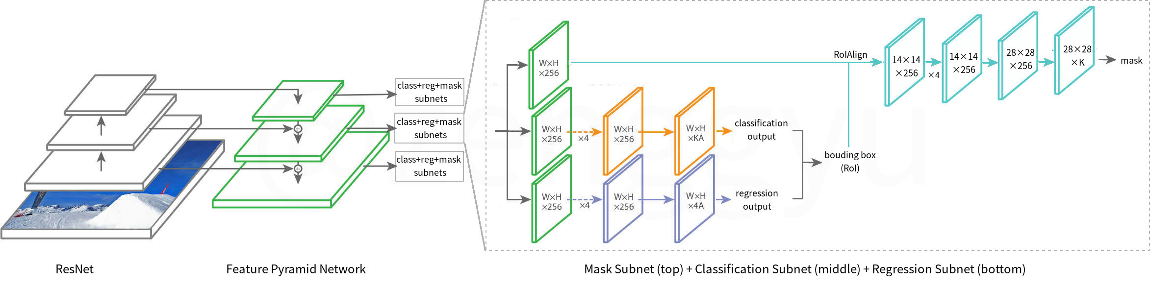
The ResNet base network, the feature pyramid network (FPN), the classification subnet and the regression subnet are identical to those of RetinaNet. Additionally, there is a mask subnet for mask prediction. Note that in this version, the subnets are directly attached to the FPN outputs (the green feature maps in the figure); this is unlike the original Mask R-CNN, where these subnets are attached to the outputs of region proposal network (RPN).
The classification subnet together with the regression subnet gives a number of bounding box predictions. Each bounding box represents a region of interest (RoI) that likely contains an instance of a certain class. Based on these predictions, the mask subnet uses a technique called RoIAlign to extract a feature map from the FPN output for each RoI, and finally applies a fully convolutional network (FCN) to predict the mask. The level (\(k\)) of the FPN pyramid whose output will be used to extract the feature map depends on the target RoI’s width and height (on the scale of the input image). Formally (Lin et al. 2017):
\[ k = \lfloor{k_0} + log_2(\sqrt{width \times height} / 224)\rfloor \quad (1) \]
where \(224\) is the canonical ImageNet pre-training size, and \(k_0 = 4\) is the target level on which an RoI with \(width \times height = 224^2\) should be mapped into.
In the following sections, I will introduce the key components of RetinaMask that is missing in RetinaNet.
RoIAlign
When performing instance segmentation, RetinaMask does not directly predict a mask that covers the whole image. Instead, it predicts one mask for each RoI that likely contains an object. To this end, for each RoI, we need to obtain a corresponding feature map to feed to the mask subnet. RoIAlign is a technique for such a purpose.
Recall that RetinaNet uses a feature pyramid network to extract feature maps of an entire image. These feature maps are then fed to the classification subnet and the regression subnet to make bounding box predictions. When building RetinaMask on top of RetinaNet, the bounding box predictions can be used to define RoIs.
The process of RoIAlign is shown in Figure 2 . By re-scaling a bounding box and projecting it to an FPN feature map, we get a corresponding region on the feature map. To obtain a new feature map within this region, we first determine a resolution. In the original paper (He et al. 2017), the resolution is set to \(14 \times 14\) (but for simplicity, the example presented in Figure 2 uses a coarser resolution, i.e., \(2 \times 2\)). For each grid cell, a number (e.g., 4) of regularly spaced sampling points are chosen, and the feature value corresponds to each point is calculated by bi-linear interpolation from the nearby grid points on the FPN feature map. For those curious, WikiPedia provides a good explanation of bilinear interpolation.
Finally, by max pooling the sampling points within each grid cell, we get the RoI’s feature map. Note that this process is not shown in Figure 2 ; but in essence, max pooling the sampling points means choosing the point with the maximum value and use that as the feature value of the grid cell. Note also that the resulting feature map has a fixed size of \(14 \times 14 \times 256\), where the number of channels (i.e., 256) is the same as that of the FPN output.
The mask subnet
After RoIAlign, each RoI feature map goes into the mask subnet ( Figure 1 ), which is an FCN. In the original paper (He et al. 2017), the FCN begins with four \(3 \times 3\) convolution layers, followed by a \(2 \times 2\) deconvolution layers with stride 22, and finally a \(1 \times 1\) convolution layer. While all hidden layers use ReLU activation, the last layers uses sigmoid activation. The size of the mask output is \(28 \times 28 \times K\), where \(K\) is the number of object classes; that is, there is a mask for every class. However, only the mask that corresponds to the predicted class is relevant in following proceses.
2 The Keras-Maskrcnn implementation (Gaiser and Liscio 2018) actually uses upsampling + convolution instead of deconvolution in this step. The intuition is explained in (Odena et al. 2016).
Computing the Loss
The mask target of an RoI is the intersection between the RoI and its associated ground-truth mask. Note that it should be scaled down to the same size as the mask subnet’s output (i.e., \(28 \times 28\)) so as to compute the loss.
The loss function for RetinaMask is a multi-task loss that combines classification loss, localization loss and mask loss:
\[ L = L_{cls} + L_{loc} + L_{mask} \quad (2) \]
The classiciation loss \(L_{cls}\) and the localization loss \(L_{loc}\) are identical to those of RetinaNet. The mask loss \(L_{mask}\) can be defined as the average binary cross-entropy loss:
\[ L_{mask} = - \frac{1}{m^2}\sum_{1 \leq i, j \leq m} [y_{ij} log \hat{y}^k_{ij} + (1 - y_{ij})log(1 - \hat{y}^k_{ij})] \quad (3) \]
where \(m = 28\) is the size of the mask output; \(y_{ij}\) is the ground-truth label (an integer of 0 or 1) of cell \((i, j)\); \(y^k_{ij}\) is the \(k\)-th mask (\(k\) is determined by the class prediction) prediction (a floating point number between 0 and 1) for the same cell.
Mask prediction
At test time, the mask subnet is only applied to the top \(n\) (e.g., 100) bounding boxes with the highest classification scores. By omitting remaining boxes, both speed and accuracy can be improved. Of the \(K\) masks predicted for one box, only the one that corresponds to the class predicted by the class subnet is used. Finally, the \(m \times m\) mask output is resized to the same scale of the bounding box in the original image, using upsampling techniques such as deconvolution and interpolation (Long et al. 2014; Jeremy Jordan 2018).