Fitting and Interpreting CART Classification Trees
Introduction
In a previous post, I introduced the theoretical foundation behind classification trees based on the CART algorithm. In this post, I will put the theory into practice by fitting and interpreting some classification trees in R.
I’ve already written a similar post on regression trees. Since there are many similarities between classification trees and regression trees, this post will focus on the differences.
About the data set
I will use a simulated data set which I introduced in a previous post as an example. The data set can be obtained using the following code:
library(tidyverse)
set.seed(1)
sample_size <- 300
dat <- tibble(
x1 = runif(sample_size, min = -1, max = 1),
x2 = rbinom(sample_size, 1, 0.5),
e = rnorm(sample_size, sd = 0.1),
p = 1 / (1 + exp(-(-2 + 3 * x1^2 + x2 + e))),
log_odds = log(p / (1 - p)),
y = rbinom(sample_size, 1, p) %>% factor()
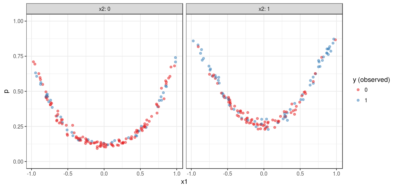
)Note that the binary outcome is stored as a factor, so that the algorithm will build a classification tree instead of a regression tree.
Figure 1 shows a visualization of the simulated data set:
Fitting classification trees on the data
Here, I use the caret::train() function to build a classification tree. No cost-complexity pruning or cross-validation is performed. The parameter that controls the minimum number of observations in terminal nodes set to 11 as opposed to 7 (i.e., the default), to reduce the size of the tree.
library(caret)
fit <- train(factor(y) ~ x1 + x2, data = dat, method = "rpart",
             tuneGrid = data.frame(cp = c(0)),
             control = rpart::rpart.control(minbucket = 11),
             trControl = trainControl(method = "none"))
The following text output describes the classification tree, which is visualized in Figure 2 .
fit$finalModel#> n= 300
#>
#> node), split, n, loss, yval, (yprob)
#> * denotes terminal node
#>
#> 1) root 300 105 0 (0.6500000 0.3500000)
#> 2) x1< 0.7342358 263 80 0 (0.6958175 0.3041825)
#> 4) x1>=-0.5097142 193 46 0 (0.7616580 0.2383420)
#> 8) x1< 0.2649135 128 24 0 (0.8125000 0.1875000) *
#> 9) x1>=0.2649135 65 22 0 (0.6615385 0.3384615)
#> 18) x2< 0.5 32 6 0 (0.8125000 0.1875000) *
#> 19) x2>=0.5 33 16 0 (0.5151515 0.4848485)
#> 38) x1>=0.3684654 22 9 0 (0.5909091 0.4090909) *
#> 39) x1< 0.3684654 11 4 1 (0.3636364 0.6363636) *
#> 5) x1< -0.5097142 70 34 0 (0.5142857 0.4857143)
#> 10) x2< 0.5 42 15 0 (0.6428571 0.3571429) *
#> 11) x2>=0.5 28 9 1 (0.3214286 0.6785714) *
#> 3) x1>=0.7342358 37 12 1 (0.3243243 0.6756757)
#> 6) x2< 0.5 19 9 0 (0.5263158 0.4736842) *
#> 7) x2>=0.5 18 2 1 (0.1111111 0.8888889) *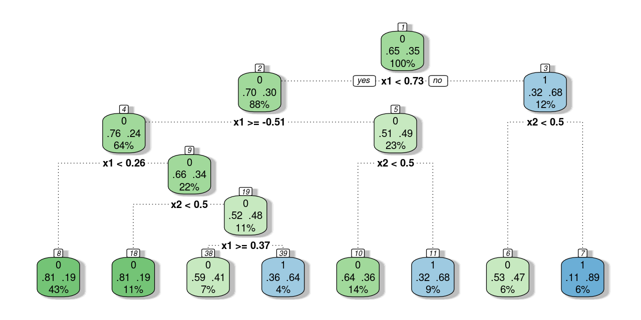
The classification tree plot is similar to that of a regression tree (see this post). The first line of text in the nodes shows the predicted outcome, and the last line of text shows the proportion of observations. However, there are some differences as well. The most apparent difference is that nodes with different predictions are filled with different colors; and the darker the color, the higher the probability of the predicted class. In addition, the middle line of text presents the probability of each class in that node.
Finally, the model is used to make predictions, which is then plotted in Figure 3 .
dat <- dat %>%
  mutate(p_predicted = predict(fit, type = "prob")[,2],
         y_predicted = predict(fit, type = "raw"))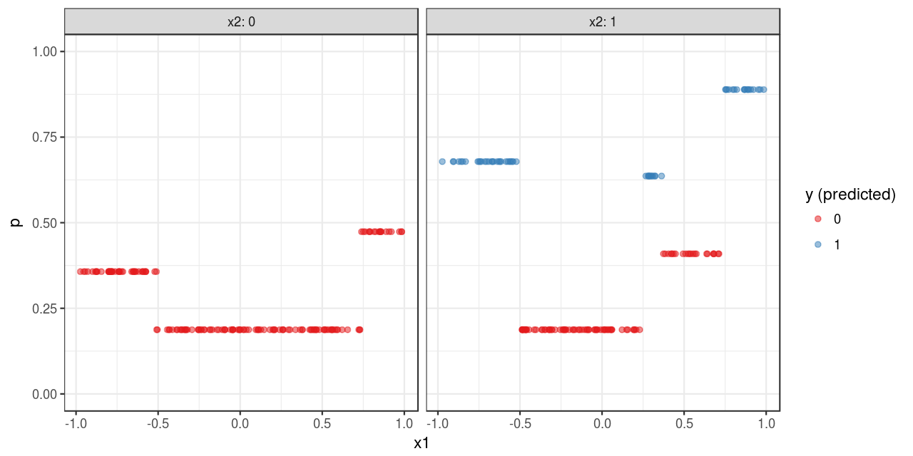
To some extent, the predictions shown in Figure 3 outlines the pattern shown in Figure 1. However, the approximation is quite rough. One reason is that CART is a non-parametric algorithm; additionally, this also have something to do with the nature of classification problems which I discussed in a previous post.
A question to be answered: how is variable importance calculated for a regression tree or a classification tree.